library(here)
library(tidyverse)
library(RColorBrewer)

# Load all the RDA files
rda_files <- list.files(path = here("data", "output", "rda"), pattern = "\\.rda$", full.names = TRUE)
lapply(rda_files, load, envir = .GlobalEnv)Explore DwC-DP
Explore the DwC-DP tables
You can load all the RDA files like below and play around with the tables as demonstrated in this page. Any pull request is also welcomed.
Community measurements
Does DwC-DP handles community measurements better than DwCA?
DwCA
In DwCA, we will have to have all these as Occurrence records so that measurements like “Standard Length” and “Total Length” of each individual in emof has an Occurrence record to point to. However, this does not warrant user to add the organismQuantity of all individuals together.
| occurrenceID | eventID | scientificName | lifeStage | organismQuantity | organismQuantityType |
|---|---|---|---|---|---|
| BROKE_WEST_RMT_051_RMT8_217697 | BROKE_WEST_RMT_051_RMT8 | Electrona antarctica | 28 | individuals | |
| AAV3FF_00231 | BROKE_WEST_RMT_051_RMT8 | Electrona antarctica | larvae | 1 | individual |
| AAV3FF_00232 | BROKE_WEST_RMT_051_RMT8 | Electrona antarctica | larvae | 1 | individual |
| AAV3FF_00233 | BROKE_WEST_RMT_051_RMT8 | Electrona antarctica | larvae | 1 | individual |
| AAV3FF_00234 | BROKE_WEST_RMT_051_RMT8 | Electrona antarctica | larvae | 1 | individual |
| AAV3FF_00235 | BROKE_WEST_RMT_051_RMT8 | Electrona antarctica | larvae | 1 | individual |
| AAV3FF_00236 | BROKE_WEST_RMT_051_RMT8 | Electrona antarctica | larvae | 1 | individual |
| AAV3FF_00237 | BROKE_WEST_RMT_051_RMT8 | Electrona antarctica | larvae | 1 | individual |
| AAV3FF_00238 | BROKE_WEST_RMT_051_RMT8 | Electrona antarctica | larvae | 1 | individual |
| AAV3FF_00239 | BROKE_WEST_RMT_051_RMT8 | Electrona antarctica | larvae | 1 | individual |
| AAV3FF_00240 | BROKE_WEST_RMT_051_RMT8 | Electrona antarctica | larvae | 1 | individual |
| AAV3FF_00241 | BROKE_WEST_RMT_051_RMT8 | Electrona antarctica | larvae | 1 | individual |
This has improved with the term eco:isLeastSpecificTargetCategoryQuantityInclusive from the Humboldt Extension. If the event has isLeastSpecificTargetCategoryQuantityInclusive = true, the count in organismQuantity of the Occurrence includes all of the larvae individuals.
DwC-DP
The Occurrence and Material are separate concepts now. We do not need to have a separate Occurrence just to indicate the total catch of a taxon. We can have a single Occurrence (total catch) with multiple Materials (individual) to indicate the total catch and preserved individuals. The measurements of the individuals (Assertions) can be directly linked to the Materials via the Material Assertion table.
event_id <- "BROKE_WEST_RMT_051_RMT8"
taxon_id <- "urn:lsid:marinespecies.org:taxname:217697"

# isLeastSpecificTargetCategoryQuantityInclusive for the Event?
survey %>% filter(eventID == event_id) %>% select(eventID, isLeastSpecificTargetCategoryQuantityInclusive)
# total catch of electrona antarctica from BROKE_WEST_RMT_051_RMT8
# because isLeastSpecificTargetCategoryQuantityInclusive = true, the count in organismQuantity of occurrenceID BROKE_WEST_RMT_051_RMT8_217697 includes the larvae from BROKE_WEST_RMT_051_RMT8_217697_Larvae
occurrence %>% filter(eventID == event_id & taxonID == taxon_id) %>%
select(eventID, occurrenceID, scientificName, lifeStage, organismQuantity, organismQuantityType)# all preserved electrona antarctica from BROKE_WEST_RMT_051_RMT8
mat <- material %>% filter(eventID == event_id & taxonID == taxon_id) %>%
select(materialEntityID, eventID, materialEntityType, scientificName, preparations)
mat# all measurements of individual electrona antarctica from BROKE_WEST_RMT_051_RMT8
mat %>% left_join(material_assertion, by = "materialEntityID") %>%
select(materialEntityID, assertionType, assertionValueNumeric, assertionValue, assertionUnit)Body part measurements
Very often, we received dataset with measurements performed on a specific body part of an organism. Example: https://www.gbif.org/occurrence/3344249657
DwC-A
It is difficult to model with DwC-A because:
- a specific body part/sample of an organism is not an Occurrence nor an Event
- it is difficult to express relationship between a Material (e.g. body part) and the Organism
- it is difficult to distinguish measurements performed on a Material or an dwc:Organism when pointing the measurement to an Occurrence record.
Currently, I modeled it using eMoF pointing to the Occurrence with body part in measurementRemarks. Specifying the body part can be embedded in a matrix of a NERC vocabulary but it is not practical to mint NERC for every body part and body part is specific to a taxon. Example: https://www.gbif.org/occurrence/3344249657
| occurrenceID | scientificName |
|---|---|
| SO_Isotope_1985_2017_1013 | Glabraster antarctica (E.A.Smith, 1876) |
| occurrenceID | measurementType | measurementValue | measurementUnit | measurementRemarks |
|---|---|---|---|---|
| SO_Isotope_1985_2017_1013 | The carbon elemental content measured in the tegument of the considered sea star specimen, expressed in relative percentage of dry mass | 12.28 | relative percentage of dry mass | tegument |
DwC-DP
Relationship between Materials can be specified through the derivedFromMaterialEntityID field. Example of a krill eaten by a fish can be modeled within a single Material table.
material %>% filter(str_starts(materialEntityID, "AAV3FF_00025")) %>%
  select(materialEntityID, derivedFromMaterialEntityID, derivationType, materialEntityType, scientificName, materialEntityRemarks)
Non-detections
DwC-A
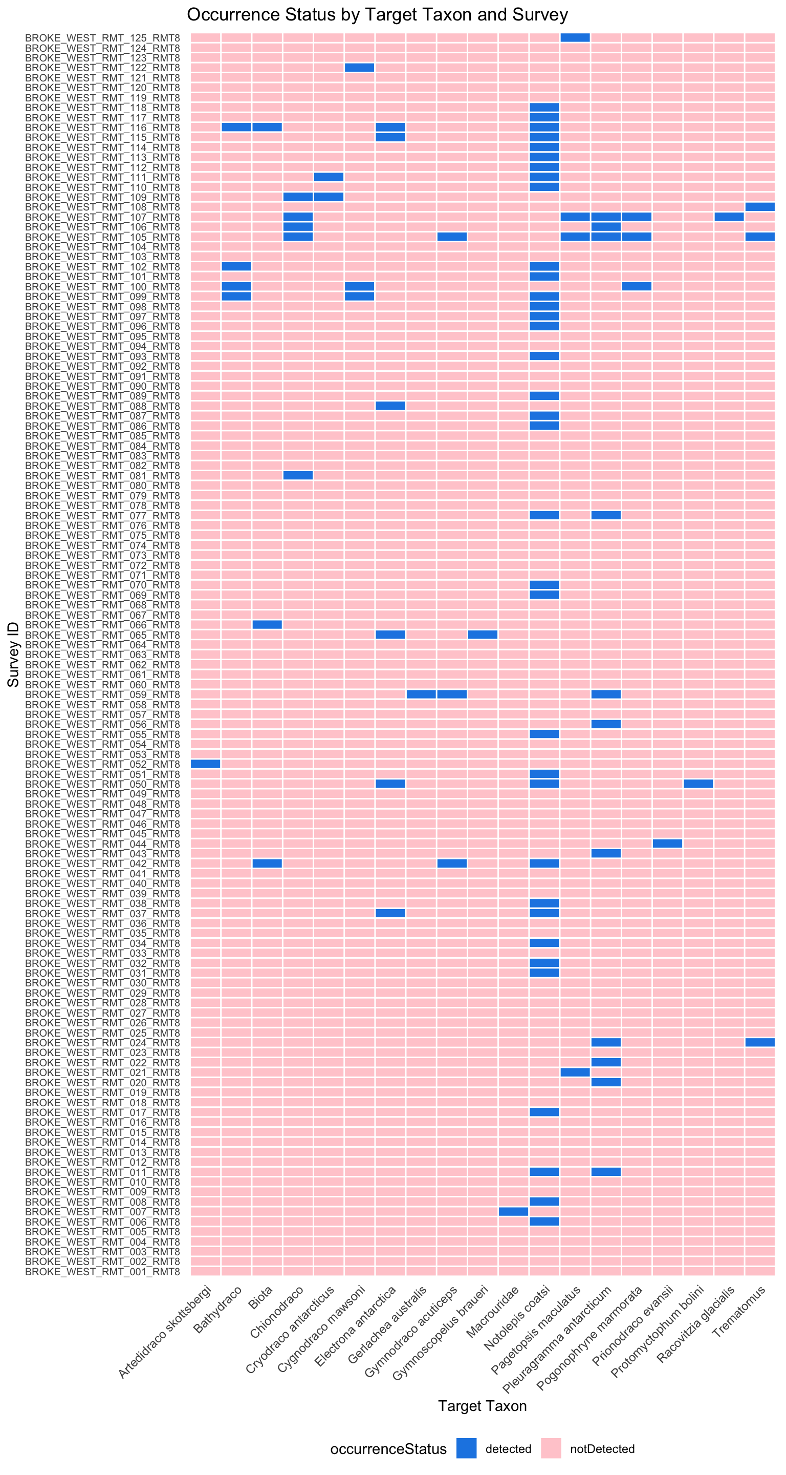
Before Humboldt Extension was developed, non-detections are represented as an Occurrence record with occurrenceStatus = absent in DwCA.
When Humboldt Extension comes along, non-detections can be inferred by looking at the target scopes that do not have an Occurrence record if the target scope was fully reported.
DwC-DP
In DwC-DP, non-detections can be represented as an Occurrence with occurrenceStatus = notDetected, just like in DwC-A. Similarly, non-detections can also be inferred by looking at the SurveyTarget that do not have an Occurrence record if only detections were reported.
library(ggplot2)

target_taxa <- survey_target %>%
  filter(surveyTargetType == "taxon") %>%
  select(surveyID, surveyTargetID, surveyTargetValue) %>%
  rename(scientificName = surveyTargetValue) %>%
  distinct()

occurrence_taxa <- occurrence %>%
  select(surveyTargetID, eventID, scientificName, eventID) %>%
  rename(surveyID = eventID) %>%
  distinct()

detections_and_non_detections <- occurrence_taxa %>%
  full_join(target_taxa, by = c("surveyID", "surveyTargetID")) %>%
  rename(targetTaxon = scientificName.y, occurrenceTaxon = scientificName.x) %>%
  mutate(occurrenceStatus = case_when(is.na(occurrenceTaxon) ~ "notDetected", TRUE ~ "detected"))

# Swap the axes so survey IDs are on the y-axis
ggplot(detections_and_non_detections, aes(y = surveyID, x = targetTaxon, fill = occurrenceStatus)) +
  geom_tile(color = "white", linewidth = 0.5) +
  scale_fill_manual(values = c("detected" = "#1F78B4", "notDetected" = "#A6CEE3")) +
  labs(
    title = "Occurrence Status by Target Taxon and Survey",
    y = "Survey ID",  # Now on y-axis
    x = "Target Taxon",  # Now on x-axis
    fill = "occurrenceStatus"
  ) +
  theme_minimal() +
  theme(
    axis.text.y = element_text(size = 7.5),  # Small text for survey IDs
    axis.text.x = element_text(size = 9, angle = 45, hjust = 1),  # Angled species names
    panel.grid = element_blank(),
    legend.position = "bottom"
  )
Length frequency diagram
DwC-DP
Can we plot length-frequency diagram of a fish species by trawl type (Target vs Routine) using the standard length measurements in DwC-DP?
# 1) lengths for Pleuragramma antarcticum
pleura_lengths <- material_assertion %>%
  filter(str_to_lower(assertionType) == "standard length" |
           str_detect(assertionTypeIRI %||% "", "SL01XX01")) %>%  # NERC SL code
  transmute(materialEntityID,
            length_mm = suppressWarnings(as.numeric(assertionValueNumeric))) %>%
  filter(!is.na(length_mm), length_mm > 0)

pleura <- material %>%
  filter(scientificName == "Pleuragramma antarcticum" |
           str_detect(taxonID %||% "", "taxname:234721")) %>%
  select(materialEntityID, eventID, scientificName)

# 2) add trawl type from event.preferredEventName
trawls <- event %>%
  select(eventID, preferredEventName) %>%
  mutate(trawl_type = case_when(
    str_detect(preferredEventName %||% "", regex("^Target", ignore_case = TRUE))  ~ "Target trawl",
    str_detect(preferredEventName %||% "", regex("^Routine", ignore_case = TRUE)) ~ "Routine trawl",
    TRUE ~ NA_character_
  )) %>%
  filter(!is.na(trawl_type))

# 3) join and plot
df_plot <- pleura %>%
  inner_join(pleura_lengths, by = "materialEntityID") %>%
  inner_join(trawls, by = "eventID")

# quick check
dplyr::count(df_plot, trawl_type)
# Bin size = 10 mm and convert counts to relative frequency (%)
ggplot(df_plot, aes(x = length_mm, fill = trawl_type)) +
geom_histogram(
aes(y = after_stat(count / sum(count) * 100)),
binwidth = 2,
color = NA,
position = "dodge"
) +
scale_fill_manual(
values = c("Routine trawl" = "#1F78B4", # blue
"Target trawl" = "#FF7F00") # orange
) +
scale_x_continuous(breaks = seq(0, 130, 10), limits = c(0, 130)) +
scale_y_continuous(expand = expansion(mult = c(0, 0.05))) +
# scale_fill_manual(values = c("#0072B2", "#E69F00")) +
labs(
title = "Size-frequency histogram of Pleuragramma antarcticum",
x = "Size class (mm)",
y = "Frequency (%)",
fill = NULL
) +
theme_bw(base_size = 12) +
theme(
legend.position = c(0.8, 0.8),
legend.background = element_blank(),
legend.key.size = unit(0.6, "lines")
)Warning: A numeric `legend.position` argument in `theme()` was deprecated in ggplot2
3.5.0.
ℹ Please use the `legend.position.inside` argument of `theme()` instead.Warning: Removed 2 rows containing missing values or values outside the scale range
(`geom_bar()`).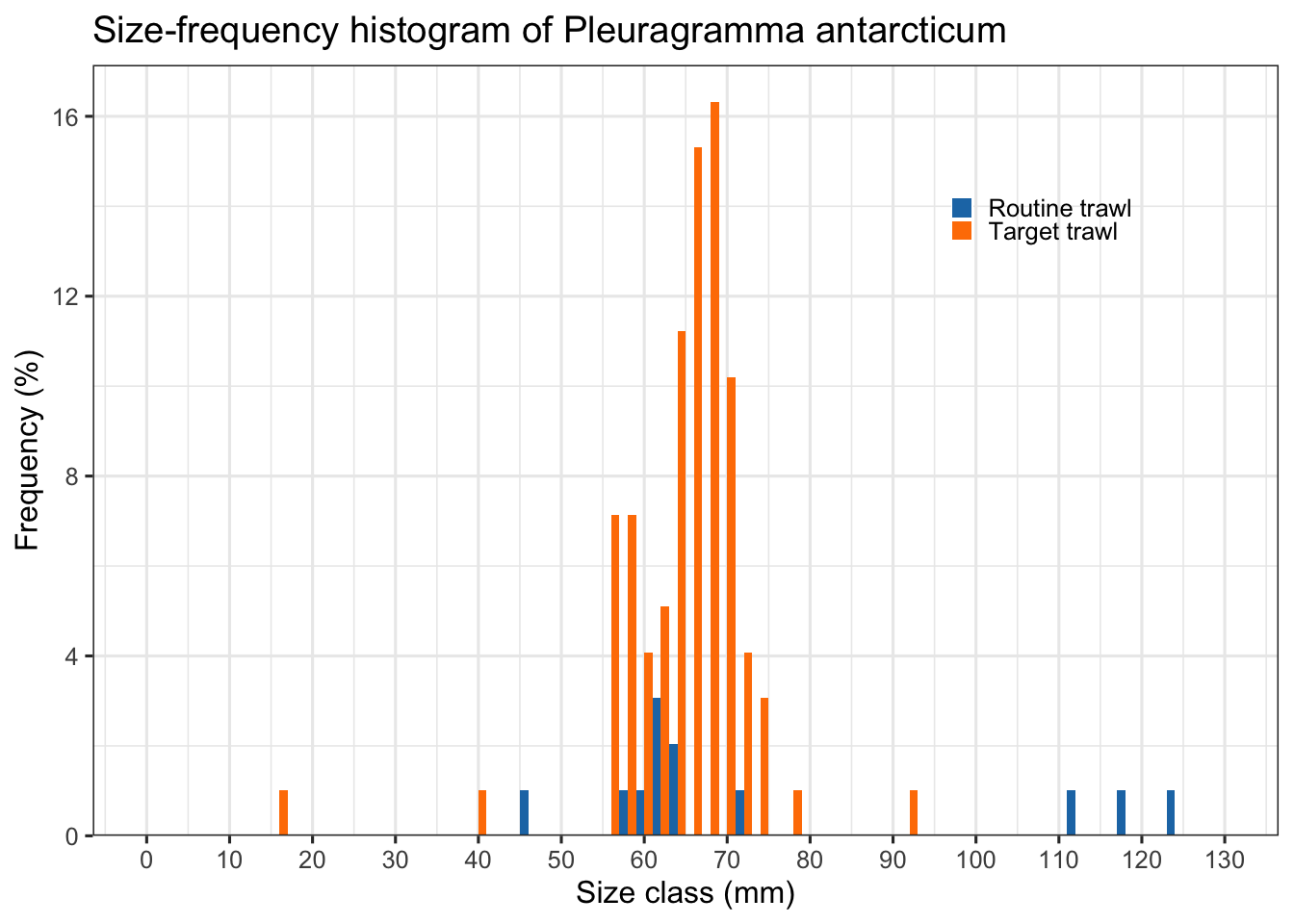
Stomach content
DwC-DP
Can we evaluate the diet composition of a fish species by trawl type (Target vs Routine) using the stomach content records in DwC-DP?
library(dplyr)
library(tidyr)
library(forcats)
library(stringr)
library(ggplot2)
library(viridisLite)  # for viridis palettes

# --- 1) Filter to stomach-content records and label prey ---
stom <- material %>%
  filter(materialEntityType %in% c("stomachContent")) %>%
  mutate(prey = if_else(is.na(verbatimIdentification) | verbatimIdentification == "",
                        "Unidentified", verbatimIdentification))

# --- 2) Add trawl type from event table ---
stom <- stom %>%
  left_join(event %>% select(eventID, preferredEventName), by = "eventID") %>%
  mutate(trawl_type = if_else(str_detect(preferredEventName, "Target"), "Target", "Routine"))

# --- 3) Collapse long tail of prey to Top N per species for readability ---
top_n <- 5

stom <- stom %>%
  group_by(scientificName, prey) %>%
  summarize(n = n(), .groups = "drop") %>%
  group_by(scientificName) %>%
  mutate(prey_rank = rank(-n, ties.method = "first"),
         prey_collapsed = if_else(prey_rank <= top_n, prey, "Other")) %>%
  select(-prey_rank) %>%
  right_join(stom, by = c("scientificName", "prey")) %>%
  mutate(prey_group = if_else(is.na(prey_collapsed), prey, prey_collapsed))

# --- 4) Compute proportional diet composition per species × trawl type ---
comp <- stom %>%
  count(scientificName, trawl_type, prey_group, name = "count") %>%
  group_by(scientificName, trawl_type) %>%
  mutate(prop = count / sum(count)) %>%
  ungroup() %>%
  group_by(scientificName) %>%
  mutate(total_n = sum(count)) %>%
  ungroup() %>%
  mutate(scientificName = fct_reorder(scientificName, total_n, .desc = TRUE))

# --- 5) Filter for Pleuragramma antarcticum ---
comp_pa <- comp %>%
  filter(scientificName == "Pleuragramma antarcticum")

# --- 6) Plot proportional diet composition by trawl type (less misleading) ---
ggplot(comp_pa, aes(x = trawl_type, y = prop, fill = prey_group)) +
  geom_col(position = "fill", width = 0.7, colour = NA) +
  scale_y_continuous(labels = scales::percent_format(accuracy = 1)) +
  scale_fill_viridis_d(option = "viridis") +
  labs(
    x = "Trawl type",
    y = "Diet composition (%)",
    fill = "Prey group",
    title = "Diet composition of Pleuragramma antarcticum"
  ) +
  theme_minimal(base_size = 12) +
  theme(
    panel.grid.major.y = element_blank(),
    legend.position = "right"
  )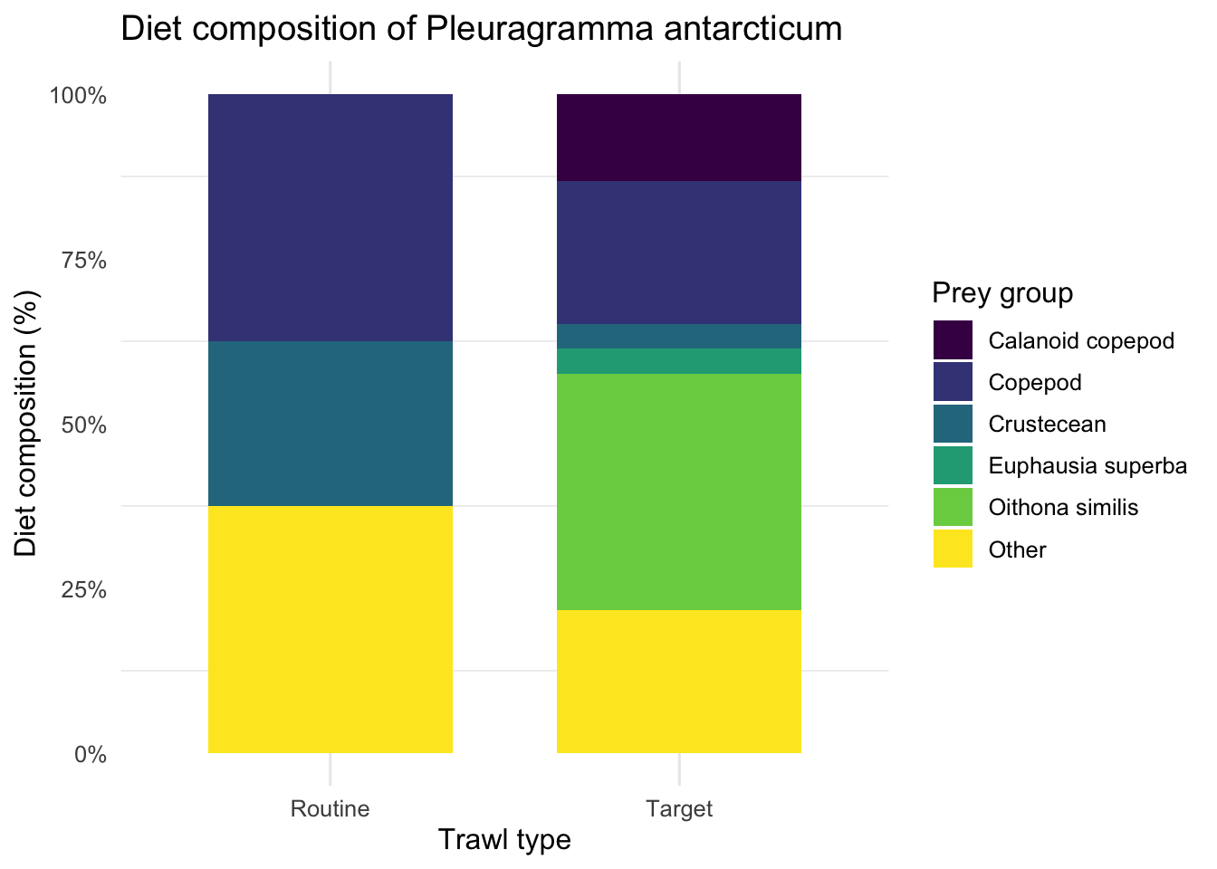
# --- 7) (Optional) Check stomach sample sizes per trawl type ---
stom %>%
  filter(scientificName == "Pleuragramma antarcticum") %>%
  count(trawl_type)